This project was completed for the Fall 2025 section of STA 610: Multilevel and Hierarchical Models at Duke University.

Overview

Street drug pricing is shaped by a complex mix of pharmacological, economic, and geographic factors. Using crowdsourced data from the StreetRx platform, this study applies hierarchical linear mixed models to analyze what drives the price per milligram (ppm) of diazepam (a benzodiazepine) and whether significant pricing variation exists across U.S. states.

Research Questions

1. Which variables are associated with the price per mg of diazepam on the street market?
2. Is there significant geographic heterogeneity in pricing across U.S. states?

Data

• Source: StreetRx — a crowdsourced database of self-reported street drug transaction prices
• Outcome: Log-transformed price per milligram — log(ppm)
• Key variables: Dosage strength (mgstr), bulk purchase indicator, information source (word-of-mouth, internet, personal), state, year
• Preprocessing: Removed primary_reason (>50% missing); excluded erroneous/outlier entries

Modeling Approach

Model Structure

where $u_j \sim \mathcal{N}(0, \sigma_u^2)$ captures state-level random intercepts — the primary quantity of interest for geographic heterogeneity.

Model Selection

An exhaustive search over 1,024 candidate models (all subsets of fixed effects) was performed using BIC as the selection criterion. The optimal model includes dosage strength, bulk purchase, source, and year as fixed effects, with state random intercepts.

Frequentist vs. Bayesian Comparison

Both approaches were implemented and compared:

Posterior distributions and REML estimates were nearly identical, providing strong cross-validation of the findings.

Key Findings

Geographic heterogeneity: The estimated between-state variance was statistically significant, confirming that state-level factors (supply chains, law enforcement, local demand) drive meaningful pricing differences. Texas was identified as a notable outlier with anomalous pricing patterns.

Model convergence: Frequentist and Bayesian parameter estimates converged nearly identically, confirming model robustness and that the data adequately inform the likelihood.

Technical Stack

• Language: R
• Packages: tidyverse, lme4, brms, rstan, kableExtra, patchwork, gridExtra, influence.ME

Full Report

This project was completed with Zhihao Chen for the Fall 2025 section of STA 522: Study Design and Causal Inference at Duke University.

Overview

Using a 2⁴ full factorial experiment, we systematically investigated which physical properties of a paper helicopter most affect flight duration — and identified the optimal design configuration for maximum airtime.

Experimental Design

We tested four binary factors across 16 treatment combinations, each replicated 5 times for a total of 80 flights:

• Response variable: Flight duration (seconds), measured from drop to landing
• Randomization: Flight order randomized within each replicate block

Statistical Methods

• Full factorial ANOVA including all main effects and two-way/three-way interactions
• Nested F-tests for model comparison and interaction significance
• Model diagnostics: residual normality (Shapiro-Wilk), constant variance (Levene’s test)
• 95% Confidence intervals for individual treatment effects

Key Findings

Interpretation: Rotor length is the most important design factor — a longer rotor increases lift and slows descent. Paper clips add weight without aerodynamic benefit, sharply reducing flight time. The significant rotor × clip interaction suggests that clipping a long-rotor helicopter is especially detrimental.

Optimal Configuration

The best-performing treatment (treatment “a”) used:

• ✅ High rotor length (8.5 cm)
• ✅ Low leg length (7.5 cm)
• ✅ Low leg width (3.2 cm)
• ✅ No paper clip

Predicted flight time: 2.47 seconds (95% CI: 2.31 – 2.63s)

Technical Stack

• Language: R
• Packages: tidyverse, dplyr, ggplot2, kableExtra

Full Report

This project was completed with Zhihao Chen for the Fall 2025 section of STA 522: Study Design and Causal Inference at Duke University.

Overview

Using publicly available data from the U.S. Department of Education’s College Scorecard, we designed and implemented a stratified random sampling study to estimate key characteristics of U.S. degree-granting institutions — without surveying all 6,000+ schools in the population.

Research Questions

1. What is the total undergraduate enrollment across all U.S. colleges?
2. What proportion of colleges offer an undergraduate Statistics major?
3. How do alumni earnings differ between public and private institutions?
4. How do annual attendance costs compare across institution types?

Sampling Design

We applied stratified random sampling with proportional allocation, dividing the population into four strata based on two binary variables:

• Population: All U.S. degree-granting institutions in the College Scorecard database
• Sample size: n = 100 institutions (proportionally allocated across strata)
• Data source: Most-Recent-Cohorts-Institution and Most-Recent-Cohorts-Field-of-Study files

Estimation Methods

For each research question, we derived design-based estimators appropriate to the quantity of interest:

• Total enrollment: Horvitz-Thompson estimator for population totals
• Proportion with Statistics major: Ratio estimator with design-based variance
• Earnings and cost comparisons: Separate ratio estimators within stratum, combined using the stratified estimator formula
• Confidence intervals: 95% CIs constructed using the normal approximation with design-corrected standard errors

Key Results

Technical Stack

• Language: R
• Packages: dplyr, ggplot2, tidyr, gridExtra, survey

Full Report

This project was completed as the final project for the Spring 2025 section of STA 663: Statistical Computing at Duke University.

Overview

Right Heart Catheterization (RHC) is an invasive diagnostic procedure widely used in ICUs — yet its causal effect on patient outcomes has long been debated. Using data from 5,735 critically ill hospitalized patients, this project estimates the Average Treatment Effect (ATE) of RHC on 30-day mortality using five different causal inference methodologies.

Dataset

• Source: RHC observational study (rhc_demo.csv)
• Sample size: 5,735 adult patients
• Treatment: RHC performed within 24 hours of admission (n = 2,184 treated; n = 3,551 control)
• Outcome: Death within 30 days of hospital admission (binary)
• Covariates: 30+ variables including demographics, diagnoses (COPD, CHF, cancer), clinical markers (PaO₂/FiO₂, WBC, temperature), and functional status (DASI index)

Methods

1. Missing Data Handling

Missing covariates were imputed using MICE (Multiple Imputation by Chained Equations) before any causal estimation.

2. Propensity Score Estimation

A logistic regression model using all 30+ covariates was fit to estimate P(Treatment = 1 | X). Overlap between treated and control propensity score distributions was verified visually.

3. Causal Estimators

4. Variance Estimation

Confidence intervals derived via bootstrap resampling and sandwich estimators for robustness.

Results

Interpretation: All five methods consistently estimate a positive ATE of ~0.040–0.045, suggesting RHC is associated with a 4–5 percentage point increase in 30-day mortality. The consistency across methods — each with different identifying assumptions — strengthens confidence in this finding.

Balance Assessment

Standardized Mean Differences (SMDs) before and after weighting were computed for all covariates. Love plots confirm that IPW and overlap weighting achieve substantially improved covariate balance relative to the unadjusted comparison.

Technical Stack

• Language: Python (Jupyter Notebook)
• Packages: pandas, numpy, statsmodels, scikit-learn, scipy, fancyimpute, matplotlib, seaborn

Full Report

This project was completed by Jessalyn Chuang, Neha Manish Shah, Michelle Schultze, and Zixiao Tan (Prairie Dog Team) for the Spring 2025 section of IDS 705: Principles of Machine Learning at Duke University.

Overview

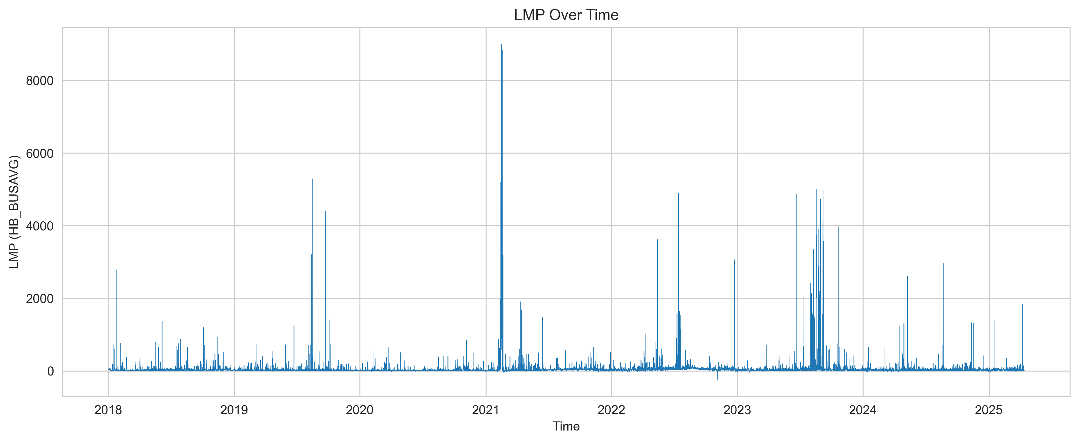
Electricity prices in wholesale energy markets are notoriously volatile, driven by demand spikes, renewable intermittency, and fuel cost fluctuations. Accurate short-term price forecasting enables grid operators, traders, and policymakers to make better decisions. This project benchmarks tree-based and deep learning models for forecasting ERCOT (Electric Reliability Council of Texas) hub prices across multiple time horizons using only publicly available data.

Target Variable

ERCOT Average Hub Real-Time Locational Marginal Price (LMP) — the wholesale electricity price ($/MWh) at the system hub, sampled hourly.

Data Sources

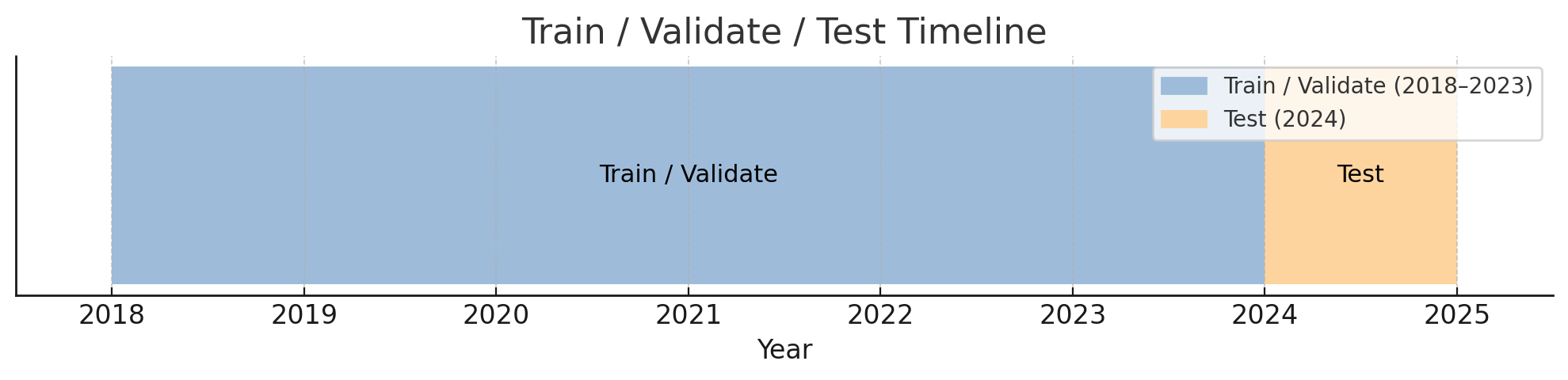
• Time period: 2018 – 2025
• Granularity: Hourly (aligned via forward-fill for daily series)
• Processed dataset: ~60,000 hourly observations after cleaning

Feature Engineering

• Lagged LMP values (1h, 24h, 168h)
• Hour-of-day, day-of-week, month cyclical encodings
• Rolling means and standard deviations of load and generation
• Wet-bulb temperature (heat stress proxy)
• Natural gas price as fuel cost signal

Models

Hyperparameters tuned using Optuna (Bayesian optimization). All models evaluated on rolling-origin cross-validation — a time-aware resampling strategy that prevents data leakage.

Results Summary

Observation: Tree-based models capture short-term autocorrelation efficiently; recurrent networks better model the multi-step temporal dependencies at the 1-day horizon.

Feature Importance (SHAP Analysis)

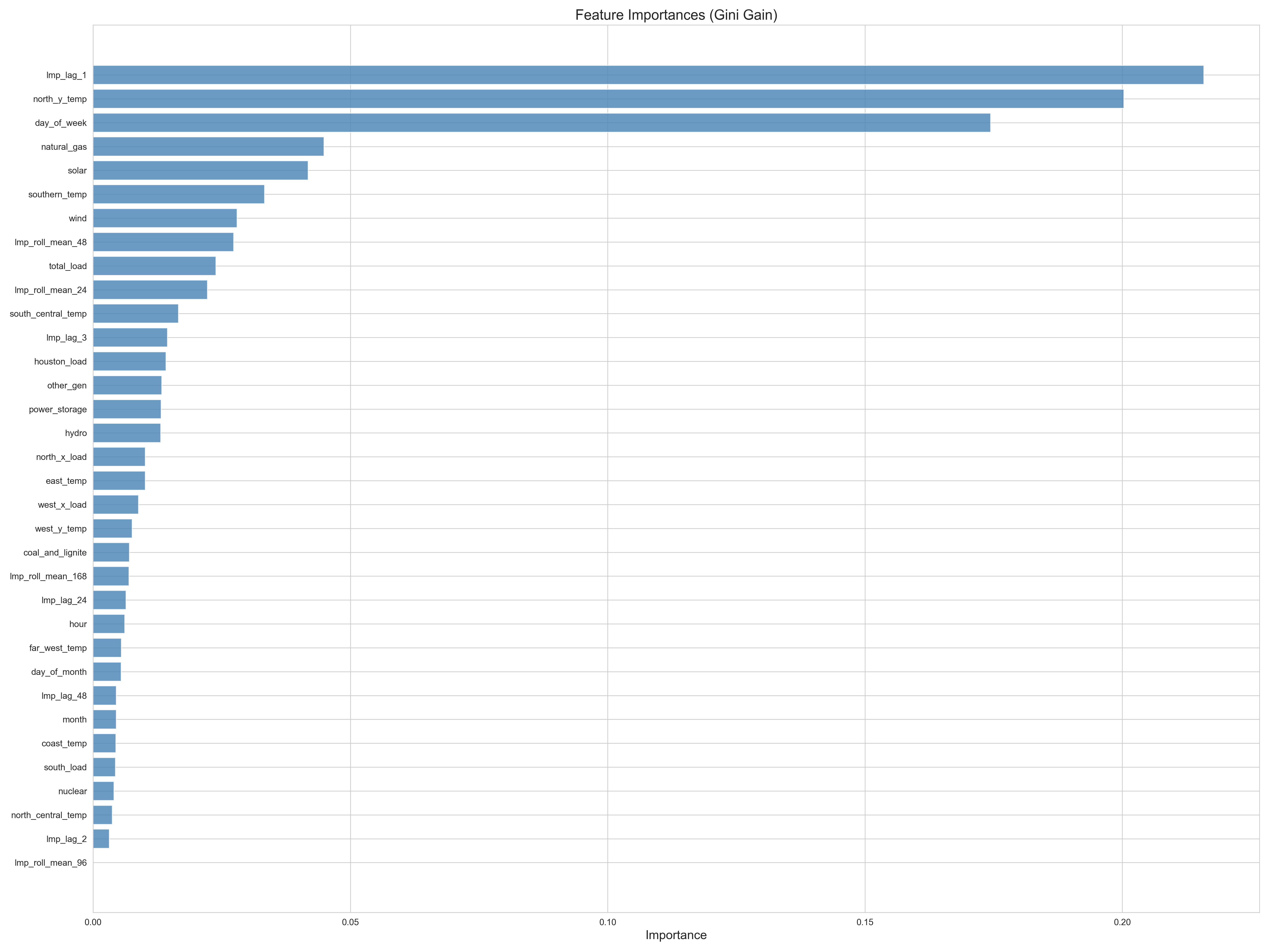
The most predictive features across all models:

1. Lagged LMP prices (1h and 24h lags) — strongest signal
2. Regional temperatures — demand-side proxy
3. Natural gas price — supply-side cost driver
4. Time-of-day features — captures intraday demand patterns

Technical Stack

• Language: Python
• ML/DL: lightgbm, xgboost, torch (LSTM/GRU)
• Optimization: optuna
• Analysis: pandas, numpy, scikit-learn, statsmodels
• Reproducibility: GitHub Actions CI for automated notebook rendering